Page 90 - Understanding NCERT Science 09

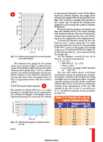
is represented along the y-axis. If the object
moves at uniform velocity, the height of its
velocity-time graph will not change with time
(Fig. 7.5). It will be a straight line parallel to
the x-axis. Fig. 7.5 shows the velocity-time
graph for a car moving with uniform velocity
–1
of 40 km h .
We know that the product of velocity and
time give displacement of an object moving
with uniform velocity. The area enclosed by
velocity-time graph and the time axis will be
equal to the magnitude of the displacement.
To know the distance moved by the car
between time t and t using Fig. 7.5, draw
1 2
perpendiculars from the points corresponding
to the time t and t 2 on the graph. The velocity
1
–1
of 40 km h is represented by the height AC
or BD and the time (t – t ) is represented by
2 1
the length AB.
Fig. 7.4: Distance-time graph for a car moving with So, the distance s moved by the car in
non-uniform speed time (t – t ) can be expressed as
2 1
s = AC × CD
–1
The distance-time graph for the motion = [(40 km h ) × (t – t ) h]
2 1
of the car is shown in Fig. 7.4. Note that the = 40 (t – t ) km
2 1
shape of this graph is different from the earlier = area of the rectangle ABDC (shaded
distance-time graph (Fig. 7.3) for uniform in Fig. 7.5).
motion. The nature of this graph shows non- We can also study about uniformly
linear variation of the distance travelled by accelerated motion by plotting its velocity–
the car with time. Thus, the graph shown in time graph. Consider a car being driven along
Fig 7.4 represents motion with non-uniform a straight road for testing its engine. Suppose
speed. a person sitting next to the driver records its
velocity after every 5 seconds by noting the
7.4.2 VELOCITY-TIME GRAPHS reading of the speedometer of the car. The
velocity of the car, in km h –1 as well as in
The variation in velocity with time for an object m s , at different instants of time is shown
–1
moving in a straight line can be represented in table 7.3.
by a velocity-time graph. In this graph, time is
represented along the x-axis and the velocity
Table 7.3: Velocity of a car at
regular instants of time

Time Velocity of the car
–1
(s) (m s ) (km h )
–1
0 0 0
5 2.5 9
10 5.0 18
15 7.5 27
20 10.0 36
Fig. 7.5: Velocity-time graph for uniform motion 25 12.5 45
of a car 30 15.0 54

MOTION 79

Rationalised 2023-24